When performing non-compartmental analysis, the area under the concentration-time curve (AUC) is calculated to determine the total drug exposure over a period of time. Together with Cmax, these two parameters are often used to define the systemic exposure of a drug for comparison purposes. For example, in bioequivalence trials, the entire statistical analysis is based on the comparison between formulations of AUC and Cmax. While the mathematics involved in the calculation of AUC are simple, there are nuances to the methods that are often misunderstood. Hopefully I can review some of the key details here. You can also view my video on YouTube.
Although AUC can be calculated directly from primary PK parameters (CL and V), I will discuss only the numerical estimation of AUC using non-compartmental analysis techniques in this blog post.
Linear Trapezoidal Method
The linear trapezoidal method uses linear interpolation between data points to calculate the AUC. This method is required by the OGD and FDA, and is the standard for bioequivalence trials. For a given time interval (t1 – t2), the AUC can be calculated as follows:
In essence the first two terms calculate the average concentration over the time interval. The last piece (t1 – t2) is the duration of time. So the linear method takes the average concentration (using linear methods) and applies it to the entire time interval. When you sum all of the intervals together, you will arrive at the total exposure from the first time point to the last. If you then divide the total AUC by the total time elapsed, you will arrive at the “average” concentration of drug in the body over the total time interval.
Logarithmic Trapezoidal Method
The logarithmic trapezoidal method uses logarithmic interpolation between data points to calculate the AUC. This method is more accurate when concentrations are decreasing because drug elimination is exponential (which makes it linear on a logarithmic scale). For a given time interval (t1 – t2), the AUC can be calculated as follows:
This method assumes that C1 > C2. The fraction represents the logarithmic average of the two concentrations. Just as with the linear method, the average concentration is multiplied by the time interval.
Linear-Log Trapezoidal Method
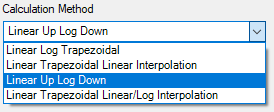
This is a combination of the first two methods and is also called “linear-up log-down”. When concentrations are increasing (as in the absorption phase), the linear trapezoidal method is used. When concentrations are decreasing (as in the elimination phase), the logarithmic trapezoidal method is used. This method is thought to be the most “accurate” because the linear method is the best approximation of drug absorption while logarithmic decline is best modeled by the logarithmic trapezoidal method during drug elimination.
Why are there different methods?
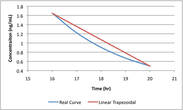
The following figure demonstrates how the linear trapezoidal method overestimates the AUC during the elimination phase. The blue line represents mono-exponential decline of a drug. Samples were drawn at 16 and 20 hours. The red line represents the linear trapezoidal methods estimation of drug concentrations. As you can plainly see, the red line is higher than the blue line suggesting overestimation by the linear trapezoidal method.
The logarithmic trapezoidal method accurately estimates mono-exponential decline of drug concentrations. However, during an absorption phase, the logarithmic trapezoidal method can underestimate the exposure.
I hope you have a better understanding of how to calculate AUC using the different methods that are available. And I hope you understand the basis of these methods and the pitfalls and limitations of each.
Today’s pharmacokineticists and PK/PD modelers are under more pressure than ever to quickly and accurately characterize the safety and efficacy profiles of investigational drugs. They need the right tools to perform non-compartmental analysis (NCA), build pharmacometric models, and generate reports that communicate their findings.
Phoenix 7.0’s new features and enhancements are the direct result of user feedback we received to make the world’s most advanced PK/PD software package even better.
Watch this webinar to learn how Phoenix 7.0 helps you handle bigger datasets, perform lightning-fast NCA, and make gorgeous plots.