Mean Residence Time: How Long Drug Molecules Stay in the Body

Ana HenryExecutive Director, Training & Certara University

April 16, 2026

When I first began learning about pharmacokinetics (PK), I was often confused by the mean residence time (MRT) parameter. I wasn’t sure what it meant, how to interpret the value, or why it would ever be important. After many years of performing pharmacokinetic analysis, I still do not use MRT very often. But I now have a better appreciation of what it is telling me so that I can use it properly, if needed.

To discuss MRT, we need to change the conversation from the concentration of drug in the body at a given time to the residence time of individual molecules in the body. The idea behind calculating the mean residence time is that each molecule spends a different amount of time in the body, with some molecules lasting a very short amount of time and others lasting longer. You can plot the relative frequency of the residence time in the body, and it looks like a concentration-time curve.

Mean residence time in pharmacokinetics

Another way to look at MRT is to use a thought experiment. Imagine we could inject exactly 10 molecules of a drug into the blood stream and then could measure when each molecule left the body. The data is presented below:

Molecule #	wdt_ID	Time in the body (min)
1	7	8.1
2	8	18.2
3	9	30.9
4	10	43.2
5	11	60.0
6	12	79.8
7	13	107.1
8	14	139.2
9	15	171.3
10	16	198.2

Note: Data from Parameters for Compartment-free Pharmacokinetics, Willi Cawello (Editor), 1999.

The half-life of the drug is the time to eliminate 50% of the drug in the body. In this case, the 5th molecule is eliminated at 60.0 minutes. The MRT is calculated by summing the total time in the body and dividing by the number of molecules, which turns out to be 85.6 minutes. Thus, MRT represents the average time a molecule stays in the body.

The generalized equation for an intravenous bolus injection is as follows:

MRT = \frac{\sum {N_i \cdot t_i}}{\sum {N_i}}

where t_i is residence time and N_i is the number of molecules with a given residence time (or all molecules for the denominator).

We can assume that every molecule that enters the body will also leave the body. So, we can substitute Dose for N_i using the following relationship:

\sum {N_i} = \int_0^{Dose} dA(t) = Dose

Finally, for drugs with linear kinetics, the amount in the body is proportional to the concentration in plasma at all time points. By making these substitutions, we can arrive at the following for MRT calculations:

MRT = \frac{\int_0^{\infty} t C(t)\,dt}{\int_0^{\infty} C(t)\,dt} = \frac{AUMC}{AUC}

where AUMC is the area under the first moment curve or the curve of concentration*time versus time.

The calculation is more complex if you have a route of administration other than IV bolus because you must account for the time required for the drug to enter the body. This is often called the mean input time (MIT). In this situation, the following equation would be used:

MRT = \frac{AUMC}{AUC} - MIT

There are many methods for estimating MIT depending on the type of dose administration.

So, why is MRT important? It can be used to estimate the average time a drug molecule spends in the body. It can also be used to help interpret the duration of effect for direct-acting molecules (e.g. blood pressure lowering agents). It should be noted that MRT is highly influenced by the measurements in the terminal phase. If there are inadequate samples to accurately estimate the terminal elimination rate constant, MRT estimates will be unreliable.

Understanding MRT calculations in Phoenix® non-compartmental analysis (NCA)

Within the Phoenix WinNonlin® NCA object, up to three mean residence time (MRT) parameters may be reported:

MRTlast
MRTINF_obs
MRTINF_pred

How these parameters are calculated depends on:

Dosing type (infusion vs. non-infusion)
Analysis type (single dose vs. steady state)

MRTlast

MRTlast represents the mean residence time from dosing to the last measurable concentration. It is only calculated for single-dose data.

Single-Dose Infusion

MRT_{\text{last}} = \frac{AUMC_{\text{last}}}{AUC_{\text{last}}} - \frac{T_{\text{inf}}}{2}

Single-Dose Non-Infusion

MRT_{\text{last}} = \frac{AUMC_{\text{last}}}{AUC_{\text{last}}}

Where:

AUMClast = Area under the first moment curve to the last measurable concentration
AUClast = Area under the concentration–time curve to the last measurable concentration
Tinf = Duration of infusion

The subtraction of Tinf accounts for drug input occurring over the infusion interval rather than instantaneously.

MRTINF (MRTINF_obs and MRTINF_pred)

MRTINF_obs and MRTINF_pred represent mean residence time extrapolated to infinity (i.e., beyond the last observed concentration time point).

MRTINF_obs uses the last observed concentration to extrapolate to infinity
MRTINF_pred uses the last predicted concentration (based on λz) to extrapolate to infinity

These parameters are calculated for both single-dose and steady-state NCA analyses, using different formulas.

Single-Dose Infusion

MRT_{\text{inf}} = \frac{AUMC_{\text{inf}}}{AUC_{\text{inf}}} - \frac{T_{\text{inf}}}{2}

Single-Dose Non-Infusion

MRT_{\text{inf}} = \frac{AUMC_{\text{inf}}}{AUC_{\text{inf}}}

Steady State Infusion

MRT_{\text{inf}} = \frac{AUMC_{\tau}}{AUC_{\tau}} - \frac{T_{\text{inf}}}{2}

Steady State Non-Infusion

MRT_{\text{inf}} = \frac{AUMC_{\tau}}{AUC_{\tau}}

Where:

AUMCINF = Area under the first moment curve extrapolated to infinity from either the last observed or last predicted concentration
AUCINF = Area under the concentration–time curve extrapolated to infinity from either the last observed or last predicted concentration
TAU is the dosing interval to steady-state
AUMC_TAU and AUC_TAU are calculated over the dosing interval
Tinf is the infusion duration

Interpretation for extravascular (oral) dosing

Lorem ipsum dolor sit amet consectetur. Donec diam risus volutpat tempor. Massa accumsan aliquam nibh tortor.Lorem ipsum dolor sit amet consectetur. Donec diam risus volutpat tempor. Massa accumsan aliquam nibh tortor dolor sit amet consectetur.Massa accumsan aliquam nibh tortor.Lorem ipsum dolor sit amet consectetur. Donec diam risus volutpat tempor.For extravascular dosing (e.g., oral models), MRTINF includes both mean input time (absorption) and time in the body after entry. Therefore, MRTINF represents the average time from dosing until a drug molecule leaves the body.

This includes:

Time required for absorption (mean input time)
Time spent in the body after entering circulation

Because these components cannot be separated without IV data, MRTINF for oral dosing should be interpreted with caution as a global residence time, rather than as time in the body after entry alone.

Hopefully, you know have a better understanding of the concept of MRT as well as how to calculate it in Phoenix WinNonlin. To learn more about pharmacokinetic concepts, get our free eBook, PK/PD Data Analysis, Concepts and Applications, 5th edition.

eBook

Deepen your PK knowledge – Free expert resource

Looking to go beyond the basics of PK parameters?

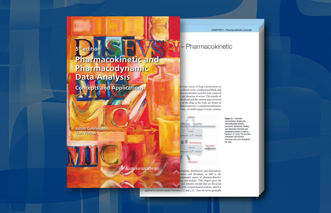
Authored by Prof. Johan Gabrielsson, the trusted reference book Pharmacokinetic and Pharmacodynamic Data Analysis provides comprehensive insights into pharmacokinetics, pharmacodynamics, and PK/PD concepts.

Get the eBook

This blog was originally published in March 2013 and has been updated for accuracy.

Author

Ana Henry

Executive Director, Training & Certara University

Ana leads the Certara University team in providing modeling and simulation for new drug development through education, skills, and expertise in the global healthcare industry. Ana has more than 20 years experience in a variety of roles in the industry. She has extensive experience in pharmaceutical training, software demonstration, software support, and product management, Ana is also an adjunct faculty member at Skaggs College of Pharmacy and Pharmaceutical Sciences at the University of Colorado.

Phoenix WinNonlin: A trusted software tool for analyzing bioequivalence and bioavailability studies 

As the industry standard for NCA, PK/PD studies, and toxicokinetic (TK) modeling, Phoenix WinNonlin delivers 30 years of reliability and innovation. Trusted by regulatory agencies like the FDA, PMDA, CFDA, and MHRA, it ensures compliance, reduces manual effort, and enhances productivity. 

Learn more

FAQs

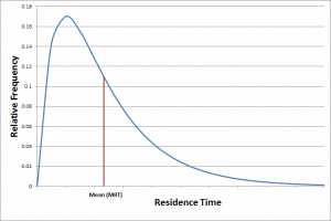
What is the difference between mean residence time (MRT) and half-life?

MRT represents the average time a drug molecule stays in the body, while half-life measures how long it takes for half of the drug concentration to be eliminated. MRT considers the full distribution of molecule lifetimes, whereas half-life focuses only on the rate of decline, making MRT more comprehensive in certain pharmacokinetic analyses.

How does poor PK sampling in the terminal elimination phase of the drug affect MRT accuracy?

Inadequate sampling during the terminal elimination phase can significantly distort MRT calculations. Since MRT relies on accurate estimation of the drug’s elimination tail, missing or sparse late-time data can lead to under- or overestimation, making the results unreliable for interpretation or decision-making.

What is the relationship between MRT and drug clearance?

MRT and clearance are inversely related when the volume of distribution is held constant. In linear pharmacokinetic systems, MRT can be expressed as Vss/CL, linking residence time in the body to both drug distribution and elimination. Specifically, MRT can be expressed as the ratio of volume of distribution to clearance in certain models. This relationship helps contextualize MRT within broader pharmacokinetic behavior, linking how long a drug stays in the body to how efficiently it is removed.

Schedule a Phoenix demo

Ready to See Phoenix in Action? Transform your PK/PD analyses with a guided demo tailored to your needs. We’ll show you how Phoenix can bridge your journey across drug development.

Industry standard PK/PD analysis

Noncompartmental analysis

Bioequivalence

Nonlinear mixed effects analysis

IVIVC toolkit

Mean Residence Time (MRT): Understanding How Long Drug Molecules Stay in the Body

Mean residence time in pharmacokinetics