


The process of curve stripping is used in both compartmental and non-compartmental analysis. Each pharmacokinetic profile is made up of one or more exponential phases. The “curve stripping” process extracts each of these exponential phases from the pharmacokinetic profile in a manual fashion that does not require non-linear curve fitting. This method was originally used to estimate pharmacokinetic parameters prior to computers. It is now used to estimate initial parameter estimates for some non-linear curve fitting programs.
To execute a curve stripping procedure, you will need a graph of the data along with a “spreadsheet” of the concentration-time data. Starting at the terminal phase of the curve (final time points with measurable concentrations), a best-fit line is drawn to the log-transformed concentration-time data. An example of this is shown in the following figure with the blue circles representing the concentration-time data and the red line the best-fit line.
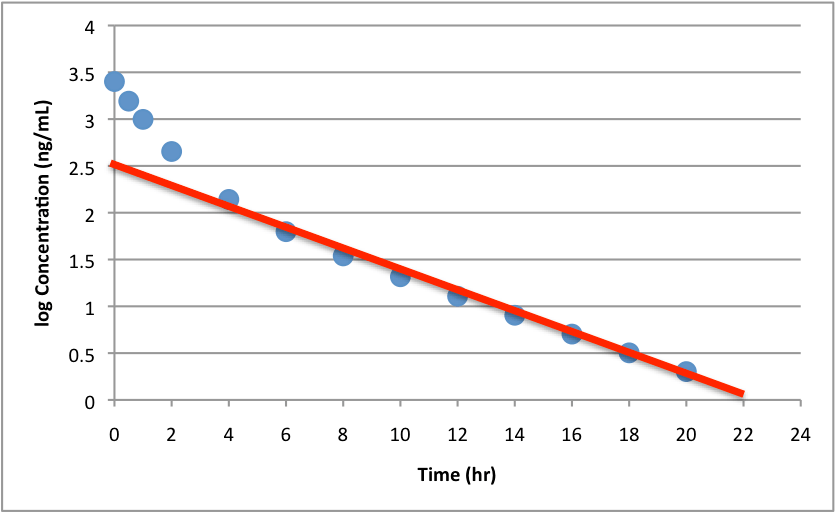
Curve Stripping Step 1
The absolute value of the slope of the red line is one of the rate constants in this biphasic pharmacokinetic curve. The second step relies in the fact that both exponential processes occur at the same time, and they are additive. The basic equation for a biphasic PK curve (with IV administration) is as follows:
=C_1*e^{-k_1*t}+C_2*e^{-k_2*t}")
The red line represents the portion of the curve explained by  , thus if we subtract that amount from the observed data (e.g.
 ") ), we will be left with the
), we will be left with the  , or the second portion of the PK curve. This then gives us our next step which requires estimating the value of the red line at time points identical to those in the early part of the curve. In this example, it corresponds to the 4 data points between 0 and 2 hours postdose. Don’t forget to back-calculate to concentration values by undoing the log transformation. This estimated concentration (red line) is subtracted from the observed concentration (blue circles) to give a new set of concentration-time data. These new data points are shown below with green circles.
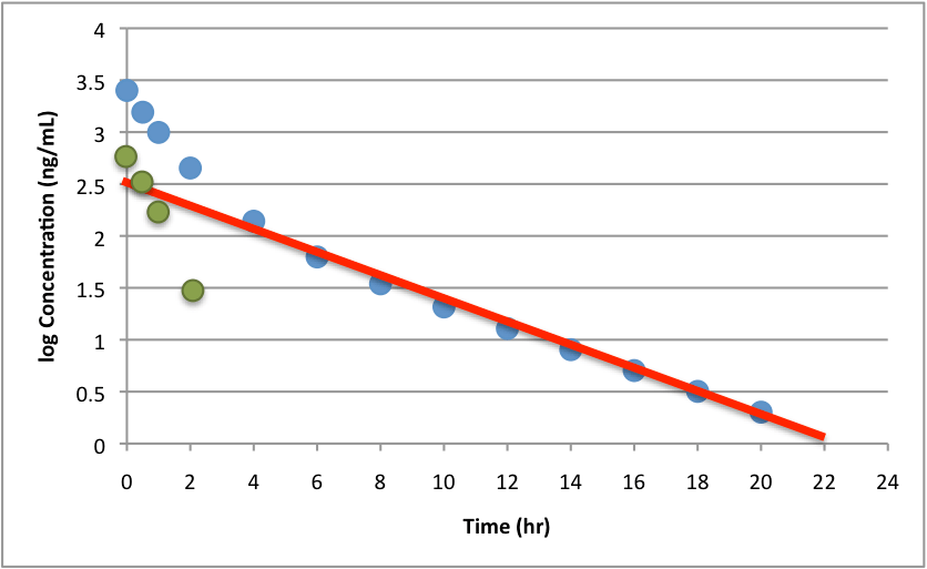
Curve Stripping Step 2
As you can see on the plot above, the green dots overlap the red line in the logarithmic scale. This is because +log(b)") . Now to determine the second exponential function, a best-fit line is drawn over the green circles. This is shown in the next figure.
. Now to determine the second exponential function, a best-fit line is drawn over the green circles. This is shown in the next figure.
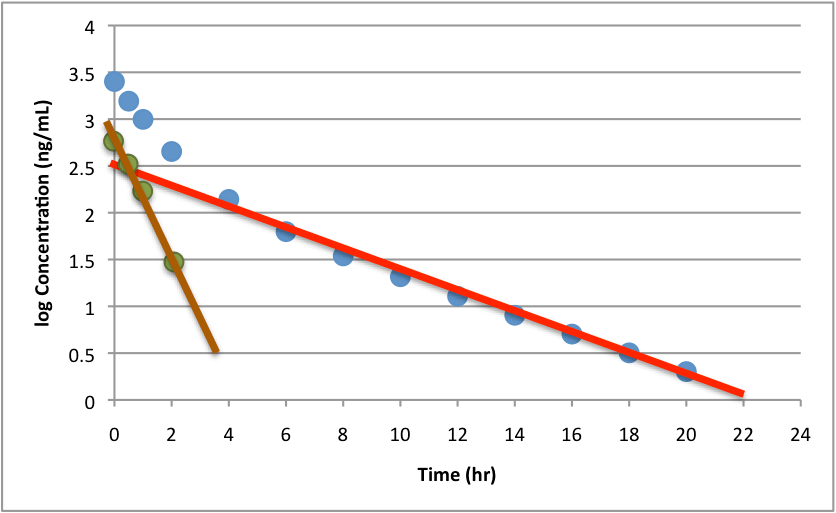
Curve Stripping Step 3
The absolute value of the slope of the second line (brownish-orange color) represents the rate constant for the second exponential in the biphasic profile. You can also estimate the coefficients  and
and  by determining where the best-fit lines cross the y-axis and then back-calculating the concentrations. From the figure above, I would estimate values of 2.4 and 2.9 for the red and orange lines respectively. This would give coefficient values of 11 ng/mL and 18 ng/mL, and the actual values were 10 ng/mL and 20 ng/mL.
Good luck stripping those pharmacokinetic curves.
The methods used to characterize the pharmacokinetics (PK) and pharmacodynamics (PD) of a compound can be inherently complex and sophisticated. PK/PD analysis is a science that requires a mathematical and statistical background, combined with an understanding of biology, pharmacology, and physiology. PK/PD analysis guides critical decisions in drug development, such as optimizing the dose, frequency and duration of exposure, so getting these decisions right is paramount. Selecting the tools for making such decisions is equally important. Fortunately, PK/PD analysis software has evolved greatly in recent years, allowing users to focus on analysis, as opposed to algorithms and programming languages. Read our white paper to learn about the key considerations when selecting software for PK/PD analysis.